The Human Nephrogenesis Atlas provides one mineable, spatially accurate transcriptomic map
of
human nephron development.
Users can explore [gene expression at single-cell
resolution], [developmental
functional networks], and [3D spatial protein domains].
A full description of this work is available [here].
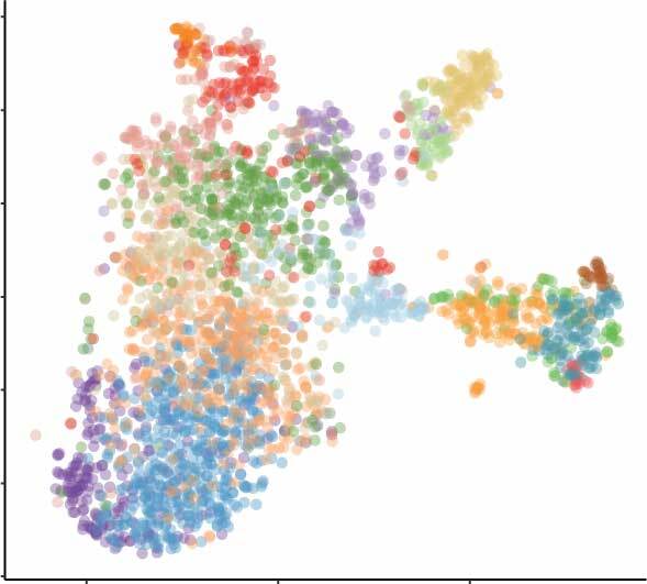
Nephrogenic single cell data
- scRNA-seq data from two week-14 human fetal kidneys (GSE139280) (read more)
- Developmental cell type and lineage identification (read more)
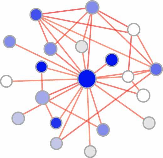
Nephrogenic gene functional network
- Identification of developmental cell type-specific genes (read more)
- Generating developmental gene functional networks (read more)
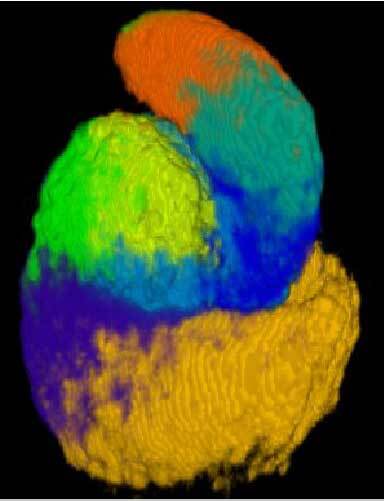
3D anatomy
- Immunofluorescent labelling and confocal microscopy imaging (read more)
- Automated image registration pipeline (read more)
- Identification of 3D spatial domains in the S-shaped body (read more)
Description
Nephrogenic single cell data
1. scRNA-seq data from two week-14 human fetal kidneys (GSE139280)
We performed scRNA-seq analyses on two week-14 kidneys (focusing on the nephrogenic niche and not
more
mature
cell-populations) obtaining 24,157 cells with a median of 2,644 genes/cell. The isolation protocol
for
single
cells from the week-14 kidneys and library construction method is described in [Lindstrom et al 2018]
. Per repeat, 7000 cells were input into the 10X
Chromium
system
and processed for single-cell library construction as per 10x Genomics instructions. Cell
transcriptomes
were
sequenced by Hi-Seq (Illumina) in 8 separate runs with ~ 120,000 reads per cell. 24,254 cells were
sequenced
to
a mean of 2644 genes per cell Quality control, mapping (to GRCh37.p13) and count table assembly of
the
library
was performed using the CellRanger pipeline version 2.1 (as consistent with 10x Genomics
guidelines). To
focus
on the most informative cells, a gene/cell count threshold of greater than 3,000, fewer than 5% of
reads
mapping
to mitochondrial genes, and a Good-Turing estimate greater than 0.7 identified 8,316 cells.
2. Developmental cell type and lineage identification
Non-cycling nephrogenic cells (2893 cells) were selected for downstream analyses and clustered using
the Seurat R package. We further
initially removed nephron
progenitor cells (CITED1+, SIX2+). The clustering was performed with 30 principal components, and
clustering explored using a range of nearest neighbour values ranging between 4 and 30, repeatedly
analyzing the differentially expressed genes between resulting clusters for segregation of known
marker genes of the predicted subdomains. We identified 3 clusters displaying a very early nephron
signature, which we termed pretubular aggregate clusters. Similarly, we identified 5 clusters that
consisted of transcriptomes from renal vesicle cells, and 6 clusters from S-shape body nephrons.
Resolved transcriptomes of differentiating cells were then remerged with three nephron progenitor
clusters for a total of 18 clusters. Cell relationships explored by SWNE [Wu et al., 2018
] showed three main trajectories corresponding to distal,
proximal, and podocyte fates, with the clusters distributed along the trajectories in an order
reflecting developmental progression. Based on marker gene analysis, the cluster annotations 1 to 18
were assigned to the resolved clusters based on developmental relationships.
Nephrogenic gene functional network
1. Identification of developmental cell type-specific genes
We develop a machine learning framework to predict functional relatedness between genes in each cell
type and developmental stage. As a first step, we identify cell-type and stage-specific genes using
Seurat. We then construct gold standards for learning functionally related genes in a cell
type-specific manner. A gene pair is labelled as cell type-specific (positive example) if both genes
are differentially expressed in this cell type, or non-specific if at least one gene is not. We
further filter the positive examples by requiring both genes in the pair to be co-annotated to a
shared GO biological process term. Gene pairs that are not both expressed in the same cell type
(could be functionally related or not) are used as negatives. These gold standards allow us to train
a classifier to predict interactive genes that are both cell-type specific and functionally related.
2. Generating developmental gene functional networks
For each developmental cell type, we predicted functional relationships across all pairs of genes. We
trained a regularized Naive Bayesian classifier by integrating labeled positive and negative gene
pairs with gene co-expression or interaction in 1,541 genome-scale data sets (including 1533 human
gene expression data sets from GEO, interaction data from BioGRID, IntAct, MINT and MIPs,
transcription factor co-regulation from JASPAR, genetic perturbation (c2:CGP) and microRNA targets
(c3:MIR) from MSigDB). A full list of datasets can be found here.
Classifier
training was performed between positive and negative gene pairs with gene co-expression or
interaction in individual data sets as features [Wong et al., 2018, using the sleipnir library].
Using the trained classifier, we predicted cell-type specific functional relatedness for every pair
of genes and presented it as an edge score
(0 ~ 1) in a weighted gene
functional network. We train a classifier for each of 18 cell types and generate 18 cell
type-specific networks.
We also generate 8 lower-resolution lineage specific networks for closely related cell types (i.e.,
nephron progenitor cell clusters 1 and 2 or cell types on the same lineage). To construct the
lineage-specific networks, we combine positive gold standards for all cell types that are part of
the lineage. We also provide a gene co-expression based network for the global developmental kidney.
To construct this network, we calculated gene co-expression across all 2893 non-cycling nephrogenic
cells using the Pearson correlation coefficient. On the Gene
Network tab of the web server, the 18
cell type networks, 8 cell lineage networks and the global network can be queried and the network
neighborhoods (genes and functional relationships) of genes of interest can be visualized.
A functional network training/prediction will take ~ 8 CPU hours. Interested users can download the
Sleipnir tool
library and input
datasets
to build gene functional networks. Data preprocessing was described in the methods section of our
paper. Pre-processed input data (~400GB) used to build developmental kidney networks can be
requested by contacting ogt@genomics.princeton.edu.
3D anatomy
1. Immunofluorescent labelling and confocal microscopy imaging
251 kidneys were labeled using immunoflorescent staining (see STAR methods for protocol). Imaging of
cortical slices (3D) was performed on a Leica SP8 using a 40X objective (40x/1.30 Oil HC PL APO
CS2). 1024x1024 images were captured at 0.35 µm optical intervals with a 1.5x zoom. Channels were
captured sequentially. Images were captured at 12-bit depth over a 0-4095 range. Care was taken to
ensure voxels were not saturated.
2. Automated image registration pipeline
We developed an
automated
image processing pipeline to process, register and combine
protein
localization assay images from renal objects allowing quantitative comparison of protein abundance.
The pipeline, written in Python, makes extensive use of both the
ANTs and
Woolz image processing
systems. Confocal images were organized into assays, with each assay composed of the set of
segmented images obtained from a single nephron. In all cases each assay contained the DAPI and
JAG1
channel images for reference, but the assays also contained a selection of two other channels
from
the set CDH1, LEF1, SALL1, SIX2, SOX9, TROMA1, WT1, LHX2, PAX2, HNF1B, FOXC2, MECOM, EMX2,
TFAP2A,
POU3F3, ERBB4, PAPPA2, CDH6, MAFB, and CLDN5. Two classes were used to group the assays of human
nephron objects for registration, namely renal vesicles and s-shaped body stage nephrons.
3. Identification of 3D spatial domains in the S-shaped body
We clustered three-dimensional protein expression patterns in order to identify developmental domains
characterized by distinct patterns of protein expression. For each protein with imaging data, we
first found the average protein expression at each voxel across all images for the protein in both
the renal vesicle and S-shaped body image sets. We then normalized across all voxels so that the
intensities of each protein had a mean 0 and standard deviation of 1 within both the renal vesicle
and the S-shaped body datasets. Selecting the set of 18 or 19 proteins with imaging data for renal
vesicle and S-shaped body respectively, we performed k-means clustering on each set of voxels,
treating each voxel as an 18 or 19 -dimensional point in genomic space. We use the k-means
implementation in the stats R package for clustering, and tested values of k ranging from 2 to 20.
We then visualized the resulting spatial patterns using Fiji, manually
removing patterns that corresponded to background noise.
On the 3D anatomy tab of the webserver, the 8 spatial domains in the
S-shaped body are interactively
visualized in 3D together with the underlying registered expression patterns of the 19 individual
proteins. Renal vesicle protein domains can be viewed in the manuscript (Figure 4).
To map developmental kidney cells to spatial domains, we imputed single-cell gene expression for the
19 proteins using the SAVER algorithm (Huang et al., 2018). For each gene, we normalized its
expression across the single-cell data. We selected 14 highly variable genes by evaluating the
expression variation across the SSB clusters. Given 8 identified protein patterns (corresponding to
the spatial domains) and adding a background pattern with zero expression of all proteins, we
computed the Euclidean distance between the gene expression vector of the 14 genes for each cell and
the corresponding protein expression vector of each pattern center, and finally assigned each cell
to the closest pattern center.
1. scRNA-seq data from two week-14 human fetal kidneys (GSE139280)
We performed scRNA-seq analyses on two week-14 kidneys (focusing on the nephrogenic niche and not more mature cell-populations) obtaining 24,157 cells with a median of 2,644 genes/cell. The isolation protocol for single cells from the week-14 kidneys and library construction method is described in [Lindstrom et al 2018] . Per repeat, 7000 cells were input into the 10X Chromium system and processed for single-cell library construction as per 10x Genomics instructions. Cell transcriptomes were sequenced by Hi-Seq (Illumina) in 8 separate runs with ~ 120,000 reads per cell. 24,254 cells were sequenced to a mean of 2644 genes per cell Quality control, mapping (to GRCh37.p13) and count table assembly of the library was performed using the CellRanger pipeline version 2.1 (as consistent with 10x Genomics guidelines). To focus on the most informative cells, a gene/cell count threshold of greater than 3,000, fewer than 5% of reads mapping to mitochondrial genes, and a Good-Turing estimate greater than 0.7 identified 8,316 cells.
2. Developmental cell type and lineage identification
Non-cycling nephrogenic cells (2893 cells) were selected for downstream analyses and clustered using the Seurat R package. We further initially removed nephron progenitor cells (CITED1+, SIX2+). The clustering was performed with 30 principal components, and clustering explored using a range of nearest neighbour values ranging between 4 and 30, repeatedly analyzing the differentially expressed genes between resulting clusters for segregation of known marker genes of the predicted subdomains. We identified 3 clusters displaying a very early nephron signature, which we termed pretubular aggregate clusters. Similarly, we identified 5 clusters that consisted of transcriptomes from renal vesicle cells, and 6 clusters from S-shape body nephrons. Resolved transcriptomes of differentiating cells were then remerged with three nephron progenitor clusters for a total of 18 clusters. Cell relationships explored by SWNE [Wu et al., 2018 ] showed three main trajectories corresponding to distal, proximal, and podocyte fates, with the clusters distributed along the trajectories in an order reflecting developmental progression. Based on marker gene analysis, the cluster annotations 1 to 18 were assigned to the resolved clusters based on developmental relationships.
1. Identification of developmental cell type-specific genes
We develop a machine learning framework to predict functional relatedness between genes in each cell type and developmental stage. As a first step, we identify cell-type and stage-specific genes using Seurat. We then construct gold standards for learning functionally related genes in a cell type-specific manner. A gene pair is labelled as cell type-specific (positive example) if both genes are differentially expressed in this cell type, or non-specific if at least one gene is not. We further filter the positive examples by requiring both genes in the pair to be co-annotated to a shared GO biological process term. Gene pairs that are not both expressed in the same cell type (could be functionally related or not) are used as negatives. These gold standards allow us to train a classifier to predict interactive genes that are both cell-type specific and functionally related.
2. Generating developmental gene functional networks
For each developmental cell type, we predicted functional relationships across all pairs of genes. We trained a regularized Naive Bayesian classifier by integrating labeled positive and negative gene pairs with gene co-expression or interaction in 1,541 genome-scale data sets (including 1533 human gene expression data sets from GEO, interaction data from BioGRID, IntAct, MINT and MIPs, transcription factor co-regulation from JASPAR, genetic perturbation (c2:CGP) and microRNA targets (c3:MIR) from MSigDB). A full list of datasets can be found here. Classifier training was performed between positive and negative gene pairs with gene co-expression or interaction in individual data sets as features [Wong et al., 2018, using the sleipnir library]. Using the trained classifier, we predicted cell-type specific functional relatedness for every pair of genes and presented it as an edge score (0 ~ 1) in a weighted gene functional network. We train a classifier for each of 18 cell types and generate 18 cell type-specific networks.
We also generate 8 lower-resolution lineage specific networks for closely related cell types (i.e., nephron progenitor cell clusters 1 and 2 or cell types on the same lineage). To construct the lineage-specific networks, we combine positive gold standards for all cell types that are part of the lineage. We also provide a gene co-expression based network for the global developmental kidney. To construct this network, we calculated gene co-expression across all 2893 non-cycling nephrogenic cells using the Pearson correlation coefficient. On the Gene Network tab of the web server, the 18 cell type networks, 8 cell lineage networks and the global network can be queried and the network neighborhoods (genes and functional relationships) of genes of interest can be visualized.
A functional network training/prediction will take ~ 8 CPU hours. Interested users can download the Sleipnir tool library and input datasets to build gene functional networks. Data preprocessing was described in the methods section of our paper. Pre-processed input data (~400GB) used to build developmental kidney networks can be requested by contacting ogt@genomics.princeton.edu.
1. Immunofluorescent labelling and confocal microscopy imaging
251 kidneys were labeled using immunoflorescent staining (see STAR methods for protocol). Imaging of cortical slices (3D) was performed on a Leica SP8 using a 40X objective (40x/1.30 Oil HC PL APO CS2). 1024x1024 images were captured at 0.35 µm optical intervals with a 1.5x zoom. Channels were captured sequentially. Images were captured at 12-bit depth over a 0-4095 range. Care was taken to ensure voxels were not saturated.
2. Automated image registration pipeline
We developed an automated image processing pipeline to process, register and combine protein localization assay images from renal objects allowing quantitative comparison of protein abundance. The pipeline, written in Python, makes extensive use of both the ANTs and Woolz image processing systems. Confocal images were organized into assays, with each assay composed of the set of segmented images obtained from a single nephron. In all cases each assay contained the DAPI and JAG1 channel images for reference, but the assays also contained a selection of two other channels from the set CDH1, LEF1, SALL1, SIX2, SOX9, TROMA1, WT1, LHX2, PAX2, HNF1B, FOXC2, MECOM, EMX2, TFAP2A, POU3F3, ERBB4, PAPPA2, CDH6, MAFB, and CLDN5. Two classes were used to group the assays of human nephron objects for registration, namely renal vesicles and s-shaped body stage nephrons.
3. Identification of 3D spatial domains in the S-shaped body
We clustered three-dimensional protein expression patterns in order to identify developmental domains characterized by distinct patterns of protein expression. For each protein with imaging data, we first found the average protein expression at each voxel across all images for the protein in both the renal vesicle and S-shaped body image sets. We then normalized across all voxels so that the intensities of each protein had a mean 0 and standard deviation of 1 within both the renal vesicle and the S-shaped body datasets. Selecting the set of 18 or 19 proteins with imaging data for renal vesicle and S-shaped body respectively, we performed k-means clustering on each set of voxels, treating each voxel as an 18 or 19 -dimensional point in genomic space. We use the k-means implementation in the stats R package for clustering, and tested values of k ranging from 2 to 20. We then visualized the resulting spatial patterns using Fiji, manually removing patterns that corresponded to background noise.
On the 3D anatomy tab of the webserver, the 8 spatial domains in the S-shaped body are interactively visualized in 3D together with the underlying registered expression patterns of the 19 individual proteins. Renal vesicle protein domains can be viewed in the manuscript (Figure 4).
To map developmental kidney cells to spatial domains, we imputed single-cell gene expression for the 19 proteins using the SAVER algorithm (Huang et al., 2018). For each gene, we normalized its expression across the single-cell data. We selected 14 highly variable genes by evaluating the expression variation across the SSB clusters. Given 8 identified protein patterns (corresponding to the spatial domains) and adding a background pattern with zero expression of all proteins, we computed the Euclidean distance between the gene expression vector of the 14 genes for each cell and the corresponding protein expression vector of each pattern center, and finally assigned each cell to the closest pattern center.